The influence of exchange rate fluctuations on Russian and Chinese export and import



Introduction

Exchange rates have a significant impact on foreign trade of different countries, acting as a communication tool between value indicators of national and global market, affecting the price ratio of exports and imports and causing a change in the domestic economic situation as well as changing the behavior of firms working in export or import competing [1].

The purpose of the work is to analyze the impact of exchange rate fluctuations on Russian and Chinese foreign trade indicators, their exports and imports.

Currently Russia's economy is largely dependent on the US dollar and the Euro. Modern state of the Russian economy can be characterized as unstable, dependent on the world market, the demand for oil, gas, nonferrous metals export. Sanctions against Russia have exacerbated the accumulated problems of real and financial sectors. As for China, in 2013, it took the leading position in the world trade. According to Chinese experts [2], China could benefit if the yuan (RMB) truly becomes a global reserve currency. In recent years, the West regularly accuses China of deliberately understating its national currency, giving an unfair advantage to Chinese exports.

Exchange rate and exchange rate policy of Russia and China are constantly in the spotlight, because currency stability and efficiency of exchange rate policy depends on the stability of the currency, which is necessary for the growth and the development of the economy.

Literature review

Consideration of the impact of currency fluctuations on the foreign trade indicators was developed in the late nineteenth century by A. Marshall [3] and continued by A. Lerner and J. Robinson. They developed the basic theoretical tenets used until nowadays. They formulates the theoretical condition under which changes of exchange rate can affect the dynamics of the trade balance [4]. Later it was called the condition of Marshall-Lerner. For the same period, works of Russian and soviet scientist Z. Katsenelenbaum [5] are related.

Later this direction was developed by S. Alexander, R. Mundell, R. Dornbusch, B. Balassa, T. Gylfason, P. Krugman, and others. In Russia authors as M. V. Ershov, S. A. Tsimailo, A. Kudrin are developing this direction. Among the empirical studies which are carried out on the level of aggregate foreign trade performance of countries, it is necessary to mention the works of T. Gylfason, P. Hooper, Wanhui Jiang, Tao Wang and in Russia P. Polivach, A. Kudrin, and others. Moreover, there are several works related to the impact of exchange rate fluctuations on the economy of the country and its competitiveness. Sample periods of studies, countries, models and selected econometric methods vary widely. The results of the works are rather contradictory.

Data collection and methodology

The chronological scope of the study covers the period from 2005 to 2016 on a monthly basis. To reach the aim of the research we use co-integration analysis of time series.

Russian total value of export, import, and inflation rates are obtained from Russian federal state statistics service. Nominal Ruble exchange rate and FDI are gathered from the Central Bank of Russia. Chinese total value of export and import, FDI and inflation rates are obtained from the National bureau of statistics of China. Nominal RMB exchange rate is obtained from the People’s Bank of China. EViews10 is used to describe the collected data, sort and analyze it.

Independent variable of the research is exchange rate of the ruble for Russia and RMB for China. Dependent variables are export and import. Additional explanatory variables are inflation and foreign direct investment.

Analysis

To check the stationarity of the series we used Augmented Dickey-Fuller test. According to the results, all series are stationary. Next, we used cointegrating framework of Johansen to test for co-integration. Table 1 illustrates the Johansen co-integration results for the relationship between exchange rate, export, import, FDI, inflation of Russia.

Table 1

Johansen cointegration test (Russia)

Hypothesized No. of CE(s)	Trace statistic	0.05Crit. Value	Prob.**
None*	111.2135	69.8188	0.0000
At most 1*	63.83538	47.8561	0.0008
At most 2	24.39237	29.79707	0.1844
At most 3	6.474454	15.49471	0.6394
At most 4	0.701027	3.841466	0.4024

Trace test indicates 2 cointegrating eqn(s) at the 0.05 level

* denotes rejection of the hypothesis at the 0.05 level

**MacKinnon-Haug-Michelis (1999) p-values

Hypothesized No. of CE(s)	Max-Eigen statistic	0.05Crit. Value	Prob.**
None*	47.37807	33.87687	0.0007
At most 1*	39.44301	27.58434	0.0010
At most 2	17.91792	21.13162	0.1329
At most 3	5.773427	14.26460	0.6425
At most 4	0.701027	3.841466	0.4024

Max-eigenvalue test indicates 2 cointegrating eqn(s) at the 0.05 level

* denotes rejection of the hypothesis at the 0.05 level

**MacKinnon-Haug-Michelis (1999) p-values

Both Trace and Maximum Eigenvalue indicate two cointegrating equations at the 0.05 level, meaning that there is at most one cointegration among variables. Therefore, we conclude that there is a long run relationship between variables. Table 2 illustrates the Johansen co-integration results for the relationship between exchange rate, export, import, FDI and inflation of China.

Table 2

Johansen cointegration test (China)

Hypothesized No. of CE(s)	Trace statistic	0.05 Crit. Value	Prob.**
None*	145.6309	88.80380	0.0000
At most 1*	78.73854	63.87610	0.0017
At most 2	39.49477	42.91525	0.1055
At most 3	18.04402	25.87211	0.3410
At most 4	4.232922	12.51798	0.7082

Trace test indicates 2 cointegrating eqn(s) at the 0.05 level

* denotes rejection of the hypothesis at the 0.05 level

**MacKinnon-Haug-Michelis (1999) p-values

Hypothesized No. of CE(s)	Max-Eigen statistic	0.05 Crit. value	Prob.**
None*	66.89235	38.33101	0.0000
At most 1*	39.24377	32.11832	0.0057
At most 2	21.45075	25.82321	0.1703
At most 3	13.81110	19.38704	0.2671
At most 4	4.232922	12.51798	0.7082

Max-eigenvalue test indicates 2 cointegrating eqn(s) at the 0.05 level

* denotes rejection of the hypothesis at the 0.05 level

**MacKinnon-Haug-Michelis (1999) p-values

Trace and Maximum Eigenvalue also indicate two cointegrating equations at the 0.05 level, which means that there is a long-term relationship among all the variables.

After cointegration test, we run Vector error correction model (VECM) to examine both the short-run and long-run dynamics of the series.

Table 3

Export (Russia)

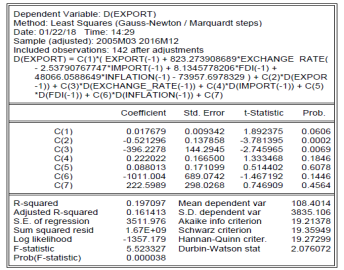
From the table above where we estimate an equation, we can see that speed of adjustment towards long-run equilibrium is positive and not significant. It means that independent variables as Exchange rate, Import, FDI and Inflation have no influence on dependent variable Export in the long run. To see the short-run causality running from independent variable to dependent one, we performed Granger causality test using Wald statistics.

Table 4

Wald test— Export

Null Hypothesis	Chi –square
	Value	Probability
There is no short run causality running from Exchange rate to Export	7.540324	0.0060
There is no short run causality running from Import to Export	1.778137	0.1824
There is no short run causality running from FDI to Export	0.264609	0.6070
There is no short run causality running from Inflation to Export	2.152653	0.1423

There is no short-run causality running from Import, FDI and Inflation to Export. Nevertheless, there is an evidence of short run causality from Exchange rate to Export.

Table 5

Import (Russia)

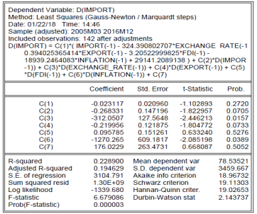
The speed of adjustment towards long-run equilibrium is negative, but it is not significant meaning that independent variables as Exchange rate, Export, FDI and Inflation have no influence on dependent variable Import in the long run. Then we performed Granger causality test using Wald statistics.

Table 6

Wald test— Import

Null Hypothesis	Chi –square
	Value	Probability
There is no short run causality running from Exchange rate to Import	5.983960	0.0144
There is no short run causality running from Export to Import	3.257203	0.0711
There is no short run causality running from FDI to Import	0.400993	0.5266
There is no short run causality running from Inflation to Import	4.348051	0.0371

There is no short-run causality running from Export and FDI to Import. However, there is an evidence of short run causality from Exchange rate and Inflation to Import.

Table 7

Export (China)

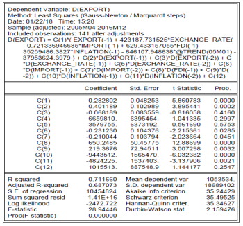
From the table above we can see that speed of adjustment towards long-run equilibrium is negative and significant. It means that independent variables as Exchange rate, Import, FDI and Inflation have influence on dependent variable Export in the long run. To see the short-run causality running from independent variables to dependent one, we performed Granger causality test using Wald statistics.

Table 8

Wald test— Export

Null Hypothesis	Chi –square
	Value	Probability
There is no short run causality running from Exchange rate to Export	1.513550	0.4692
There is no short run causality running from Import to Export	6.226055	0.0445
There is no short run causality running from FDI to Export	203.6682	0.0000
There is no short run causality running from Inflation to Export	36.75546	0.0000

There is no short-run causality running from Exchange rate to Export. Nevertheless, there is an evidence of short run causality from Import, FDI and Inflation to Export.

Table 9

Import— China

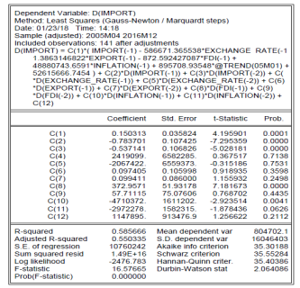
The speed of adjustment towards long-run equilibrium is significant but not positive meaning that Exchange rate, Export, FDI and Inflation have no influence on Import in the long run. To see the short-run causality, we performed Granger causality test using Wald statistics.

Table 10

Wald test— Import

Null Hypothesis	Chi –square
	Value	Probability
There is no short run causality running from Exchange rate to Import	0.215828	0.8977
There is no short run causality running from Export to Import	53.93895	0.0000
There is no short run causality running from FDI to Import	72.38900	0.0000
There is no short run causality running from Inflation to Import	9.021986	0.0110

There is no short-run causality running from Exchange rate to Import. There is an evidence of short run causality from Export, FDI and Inflation to Import.

Discussion of the results

According to the empirical tests, we did not find the evidence of influence of ruble exchange rate on export and import in the long period. However, it has an impact on export and import in the short run. The volume of exports and imports declined significantly in 2008 and 2014–2015. In 2008 there was a decline due to the financial crisis around the world. Nevertheless, it is important to notice about sharp decline in the volume of export and import and sharp devaluation of the ruble in 2014–2015. In the second half of 2014 there was a dramatic collapse in oil prices. The reason for the negative impact of falling oil prices on exchange rate is the high share of oil exports in total exports. One-third of total exports of goods exported to the CIS and other countries is oil. While the share of raw material industries in Russian exports remains significant, so fluctuations in world prices for commodities will provide a strong weakening or strengthening effect on the ruble exchange rate regardless of the country’s currency policy. That is why this situation affected the decline of the volume of export.

If the decline in exports of goods is connected to falling of oil prices, the decline in imports is happened due to the current political events, particularly sanctions in the form of an embargo on the importation of certain goods from the European Union. However, in the long run the effect will still be positive due to the import substitution. The price of oil and the imposition of sanctions on Russia by European countries, Canada and some other developed countries affects the exchange rate of the ruble. In turn, the devaluation of the ruble had an impact on the volume of export and import, but only in the short run.

Central Bank of the Russian Federation intends to adhere to such a policy in the exchange rate as following the market trends without a significant interference of authorities of monetary regulation in the exchange rate. In our opinion, it best fits the purposes of long-term economic development of Russia. However, the share of raw-material industries in Russian exports remains significant, so fluctuations in world prices for raw materials will provide a strong weakening or a strengthening effect on the exchange rate regardless of the country’s currency policy. Therefore, it would be advisable to pay more attention to other factors that can contribute to sustainable growth of exports and improves the trade balance of the country. The most important among them is the development of a competitive environment and creation of favorable business climate.

As for China, we found out that exchange rate of the RMB does not affect import nor in the short run neither in the long run. Moreover, it has no impact on export in the short run, but it influences it in the long period. It is interesting to note that FDI and inflation affected export in the long run as well as in the short run, and import in the short run. Besides, the causal links between export and import are bidirectional; they effect each other in the short run. It is bidirectional because processing trade in China occupies a large part of exports, while raw materials and intermediate goods of such kind of a trade mostly depend on imports. That is why the growth of exports will indeed lead to the growth of imports.

According to the results, RMB exchange rate does not influence import. It is because of the other factors that have an impact on it greater than exchange rate. For example, the development of the Chinese economy and growing demand in the domestic market stimulate the import trade growth. We found out that RMB exchange rate had an impact on export in the long period. Many Western partners criticized Beijing for excessive regulation of the exchange rate and stimulating exports due to the undervalued currency. According to analysts, one of the main reasons of devaluation is an attempt to increase the competitiveness of Chinese products in international markets. For China, devaluation of the yuan means increasing of exports, respectively, of revenues from exports. However, it raises another question so called “trilemma”. In 2014 because of the capital outflow China has tightened control over the movement of capital, publicly stating on the return of the RMB exchange rate to normal levels. Nevertheless, China seeks not to stop the weakening of the RMB, but only to control it. Too sharp depreciation may cause a jump in inflation and trigger the uncontrolled outflow of capital. Also due to the weakening of the RMB, Chinese companies will find it harder to service debts in foreign currencies. But attempts to stabilize RMB threaten other aspects of financial stability of China.

China is developing its strategy currency regime based on the characteristics of its economic growth. China has its own schematic view of the solution to global currency issues, the essence of which is to make the Chinese RMB a reserve currency. At the same time, China should take measures to reduce the share of the dollar in foreign exchange reserves and increase the shareholding of other currencies.

References:

1. Holopov A. Exchange rate as an instrument of macroeconomic regulation [J]. World economy and international relations, 2004, 12: 25–33.
2. Jiachun Huang, Yuping Lan. An empirical analysis of the influencing factors of RMB exchange rate [J]. Emergence and Transfer of Wealth, 2017, 7 (1).
3. Marshall A. Money, Credit and Commerce [M]. L.: McMillan, 1923, 385 p.
4. Lerner, A. The Economics of Control: Principles of Welfare Economics [M]. N.Y.: A. M. Kelley, 1975, 428 p.
5. Katsenelenbaum Z. Depreciation of the ruble and prospects for money circulation [M]. Moscow, 1918, 66 p.