1. Introduction
We consider numerical solving the hyperbolic equation
equipped with suitable initial condition for known velocity coefficient

Among the successful numerical methods for solving this equation we mention such nonoscillatory conservative finite difference shemes as TVD (total variation diminishing), TVB (total variation bounded), and ENO (essentially nonoscillatory) ones (see, for example, [1]- [14] and the reference there).
In order to highlight the essential ingredients of suggested approach we begin with one-dimensional problem, keeping in mind that we shall extend these methods in subsequent papers. Moreover, for simplification we take periodic data to avoid a description complication for inessential issues connected with boundary-value conditions.
2. The statement of problem and the main theorem
Thus, in the rectangle
 consider equation
with initial condition
Coefficient
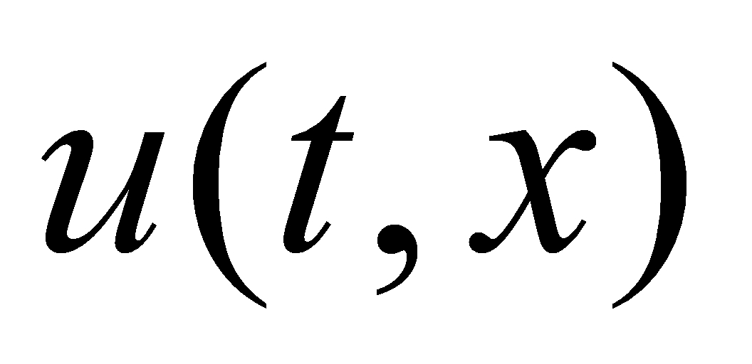 is given at
 and functions
 are supposed periodical in
 with period
 and are smooth enough for further considerations.
One of difficulties in solving (1)-(2) is that solution may contain discontinuities even for smooth data. But we start our considerations for the case of smooth solution.
Let us take two time lines
 with
with
 and two nodes

For both these nodes we construct the characteristics
 of equation (1) at segment
 [16, 17]. They satisfy the ordinary differential equation with
different initial values:
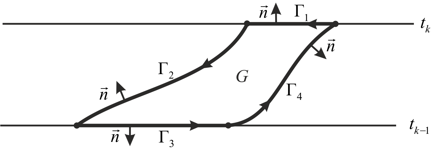
Fig. 1. Trajectories
These characteristics define two trajectories for
 in plane
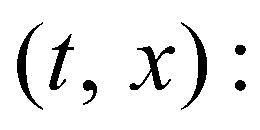
 Each of these trajectories crosses line
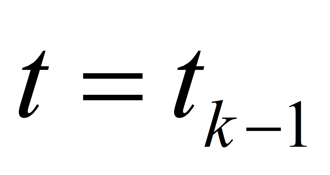 in some point
 We suppose that they are not mutually crossed and therefore

Theorem 1. For smooth solution of equation (1) we have equality
Proof. Define by
 the curvilinear quadrangle bounded by lines
 And define by
 the corresponding parts of these lines, which form the boundary
 (see Fig. 2). Introduce also the external normal
 defined at each part of boundary except 4 vertices of quadrangle.
Now use formula by Gauss-Ostrogradskii [16, 17] in the following form:
where sing
 means scalar product. Since the boundary
 consists of four parts we calculate the integral over
 separately on each line:
Fig. 2. Integration along boundary
Along the line
 the
external normal equals
 Then
ThenMinus appeared in right-hand side because of opposite direction of integration. At arbitrary point
 the tangent vector is
 Therefore the external normal equals
Therefore we get
For other two parts of the boundary we use the same way to calculate the integrals and get
Combine (5) — (7) and (9) — (11):
It implies (4). □
3. Simple semi-discrete approximation
Now take integer
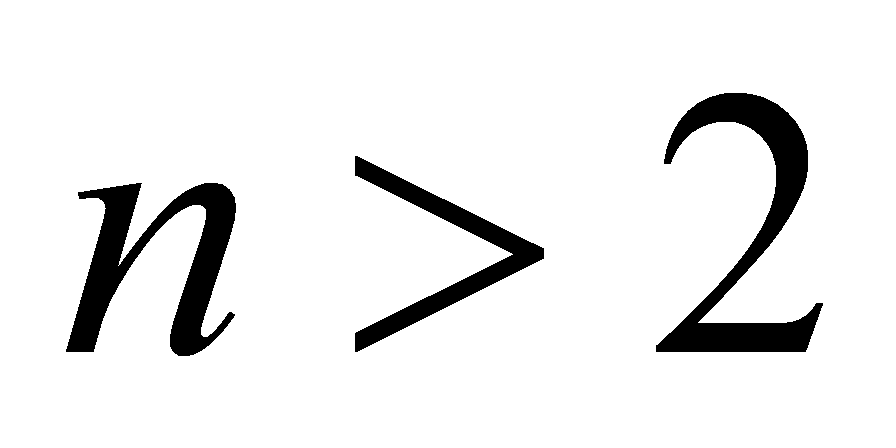 and construct uniform mesh in
 with nodes
 and meshsize
 Let we know the (approximate) solution
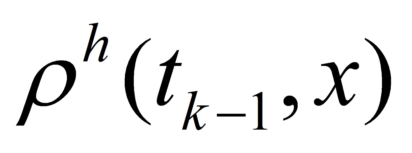 at time level
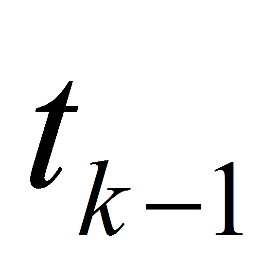 and construct the approximate solution at time level
 Integrals of solution in a small vicinities of each point
 may be some useful intermediate data. For example, let construct
integrals
may be some useful intermediate data. For example, let construct
integralsFor this purpose in the context of previous section we take two points
 and construct two trajectories
 These trajectories produce two points
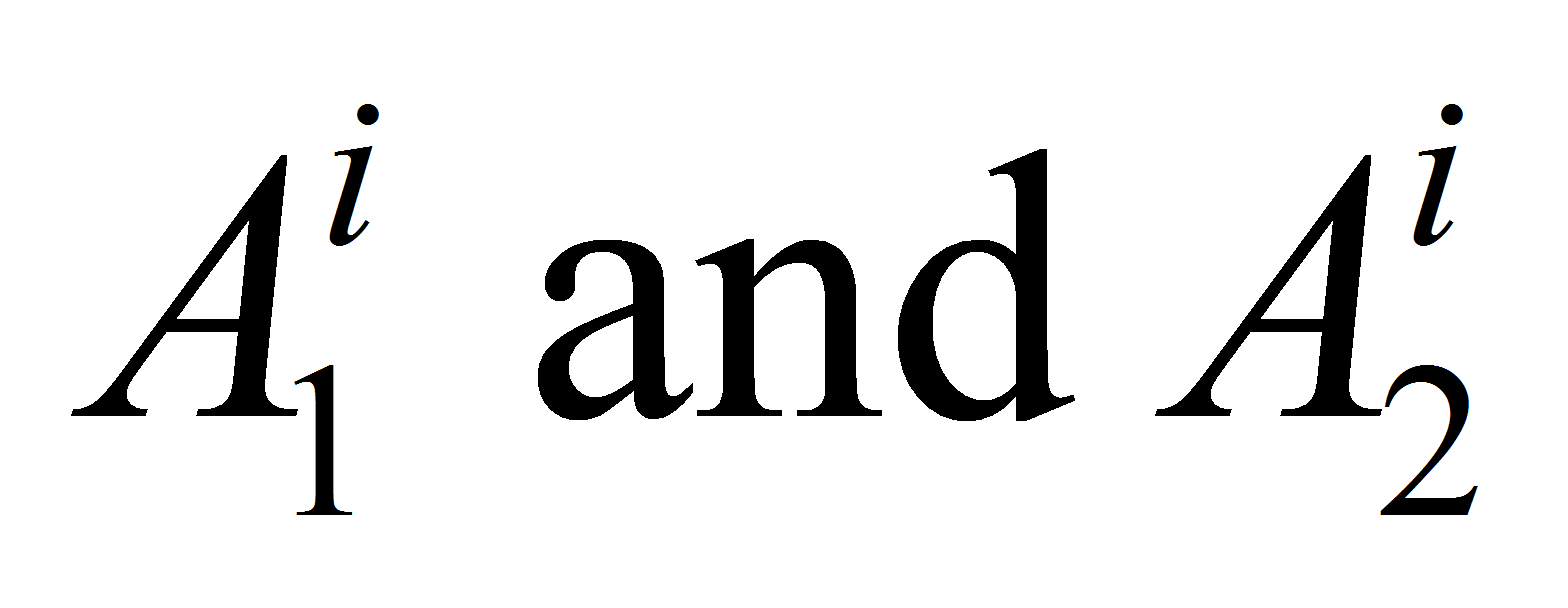 at time level
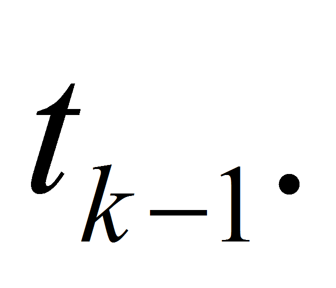 Due to Theorem 1 we get
Fig. 3. Segment for partial integration on grid
But at previous level we know only integrals on segment
 which generally do not coincide with segment
 For example, let we have situation at level
 with some integer
 as in Fig. 3. So, we need to use some approximation of partial
integrals.
as in Fig. 3. So, we need to use some approximation of partial
integrals.The simple way consists in approximation of solution by piece-wise constant function. Thus we put
But this interpolation is rather rough. It gives accuracy of order
 only. Instead of it we take linear interpolation at each segment
 For this purpose at first we put
and then define
with period
 for
for
 This time we get interpolation accuracy of order

Of course the situation at initial level
 is
simpler: we can use for example trapezoidal quadrature formula for
any segment
 with accuracy

Therefore our numerical algorithm for solving problem (1) — (2) is as follows. Take integer
 and construct uniform mesh in
 with nodes
 and meshsize
 Then for
 make the following cycle supposing that the approximate solution
 is known yet at previous time-level for

1. With the help of values in these points and periodicity we construct the piecewise linear (periodical) interpolant
2. For each point
 construct trajectories
 down to time-level
 like in previous considerations. They produce cross-points
 If
If
 goes outside segment
 we use periodicity of our data.
2. For each interval
 compute integral
by trapezoid quadrature formula separately at each nonempty subinterval
 where
where
 is linear.
3. Due to Theorem 1 it is supposed that
Therefore like in (15) — (16) we put
Thus, we complete our cycle which may be executed up to last time-level

Condensed form of this algorithm in terms of piecewise linear periodical interpolants is written as follows:
So, we get approximate discrete solution
 at each time-level
 First we prove the conservation law in discrete form.
Let a discrete function
 is given, and we construct piecewise linear interpolant
 with period 1.
Theorem 2. For any initial condition
 the approximate solution (17) —
(20)
 satisfies the equality:
Proof. We prove this equality by induction in
 For
For
 this inequality is valid because of initial condition. Suppose that
estimate (21) is valid for some
 and prove it for
 Indeed, because of (18) and (20) we get
And due to periodicity of function

Thus we prove
Now we prove a stability of algorithm (17) — (20) in the discrete norm analogous to that of space

Theorem 3. For any intermediate discrete function
 the solution
 of (17) —
(20) satisfies the inequality:
of (17) —
(20) satisfies the inequality:Proof. Indeed, because of (18) and (20) we get
Due to periodicity of functions
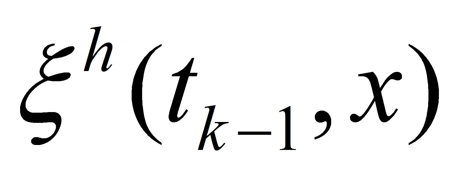 and
and
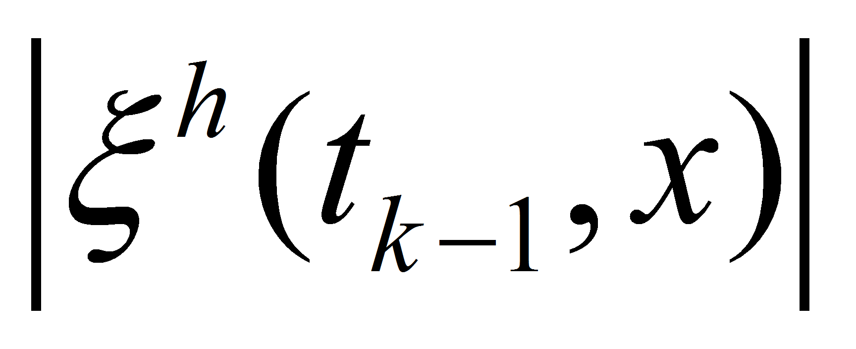
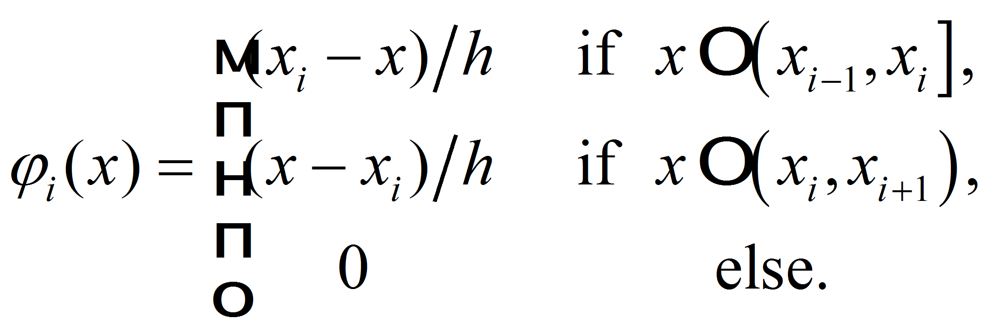
Let introduce the basis functions for linear interpolation
Then for piecewise linear interpolant we get
Then
Combine this inequality with (25) and (26) we get (24). □
Now evaluate an error of approximate solution in introduced discrete norm.
Theorem 4. For sufficiently smooth solution of problem (1) — (2) we have the following estimate for the constructed approximate solution:
with a constant
 independent of

Proof. We prove this inequality by induction in
 For
For
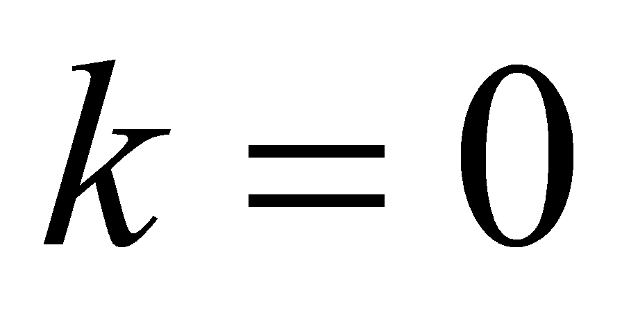 this inequality is valid because of exact initial condition (2):
 Suppose that estimate (26) is valid for some
 and prove it for

So, at time-level
 we
have decomposition
we
have decompositionwith a discrete function
 that satisfies the estimate
Because of Taylor series in
 of
of
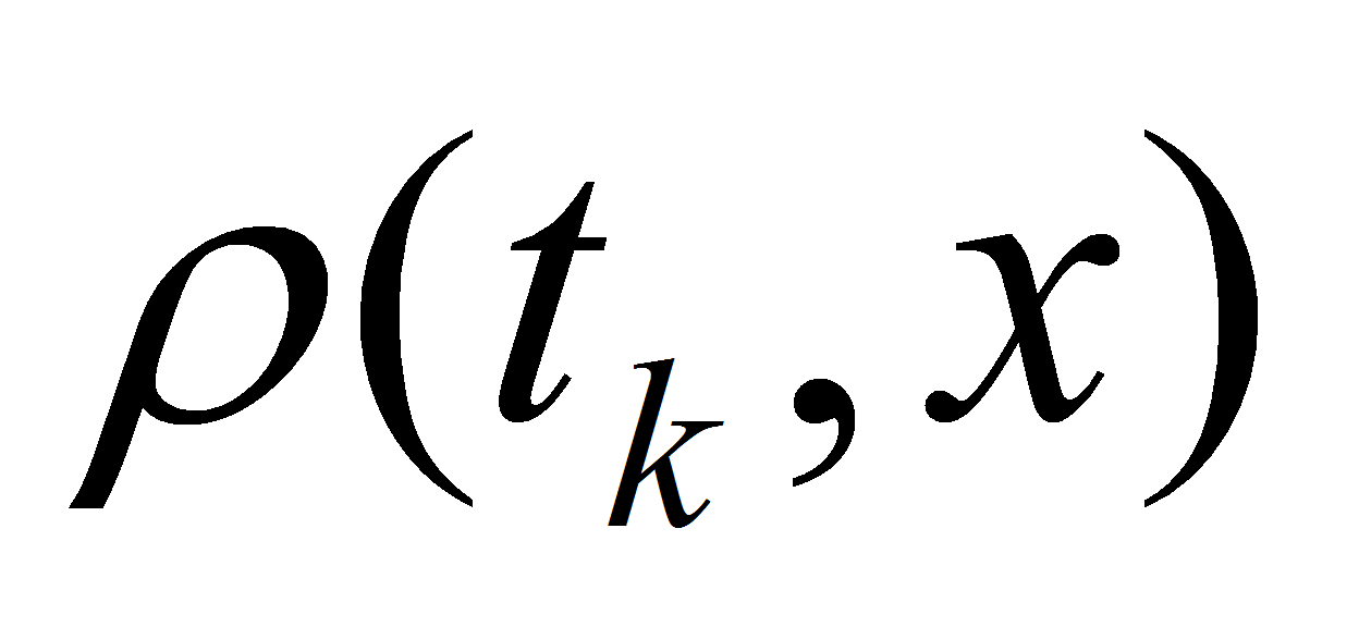 in the vicinity of point
 we get equality
Because of Theorem 1
Instead of
 let use its piecewise linear periodical interpolant
 Then
ThenThus, we get equality
where values of
 are constructed by piecewise linear periodical interpolation.
Now let subtract (33) from (32), multiply its modulus by
 and sum for all

Due to Theorem 3 last terms in brackets is evaluated by
 Thus
ThusLet put
 then this inequality is transformed with the help (29):
that is equivalent to (27). □
We can see that at last level we get inequality
In some sense we got a restriction on temporal meshsize
 to get convergence. For example, to get first order of convergence,
it is enough to take
to get convergence. For example, to get first order of convergence,
it is enough to takewith any constant
 independent of
 But this restriction is not such strong up to constant as Courant —
Friedrichs — Lewy (CFL) condition:
But this restriction is not such strong up to constant as Courant —
Friedrichs — Lewy (CFL) condition:Moreover, it is opposite in meaning: here the greater
 the better accuracy.
Thus, this approach is convenient for the problems with huge velocity
 which come from a computational aerodynamics: we have
computational stability on the base of Theorem 3 and conservation
law on the base of Theorem 2.
which come from a computational aerodynamics: we have
computational stability on the base of Theorem 3 and conservation
law on the base of Theorem 2.4. Numerical experiment
Let take
 and solve this equation with initial condition
Then exact solution is
The result of implementing the presented algorithm is given in Table 1 for several
 The first column of Table 1 expresses a relation
 /
h
(for most implemented values in computations) and the first string
shows a number n of
mesh nodes. Other entries contain the value

Table 1
|
n |
64 |
128 |
256 |
512 |
1024 |
2048 |
|
4 |
0,02358 |
0,01203 |
0,00608 |
0,00305 |
0,00153 |
0,00077 |
|
2 |
0,04536 |
0,02360 |
0,01204 |
0,00608 |
0,00305 |
0,00153 |
|
1 |
0,08423 |
0,04546 |
0,02362 |
0,01204 |
0,00608 |
0,00305 |
|
1 / 2 |
0,14610 |
0,08442 |
0,04548 |
0,02362 |
0,01204 |
0,00608 |
|
1 / 4 |
0,22493 |
0,14643 |
0,08446 |
0,04549 |
0,02362 |
0,01204 |
Thus we indeed have the first order of accuracy on h when
 /
h is
fixed.
/
h is
fixed.5. Conclusion
Thus, we present the numerical approach which is more convenient for huge velocity
 then approaches listed in introduction. Of course, we stay some open
questions like boundary condition instead of periodical one,
nonlinear dependence of velocity
 on solution
 and other. Of course, we need to trace the effect of the approximate
solving the characteristics equations instead of exact process. But
we successively consider these issues in next publications,
including generalization for two-dimensional and three-dimensional
equations.
and other. Of course, we need to trace the effect of the approximate
solving the characteristics equations instead of exact process. But
we successively consider these issues in next publications,
including generalization for two-dimensional and three-dimensional
equations.At first glance, this approach is some integral version of the characteristics method. Moreover, its accuracy is higher, the less time steps done in the algorithm. But in the future, we will apply it to the equations with nonzero right-hand side for the approximation of which a small time step
 will be crucial.
References:
Harten A.: On a class of high resolution total-variation-stable finite-difference schemes // SIAM J. Numer. Anal. — 1984. — V. 21. — P. 1–23.
Harten A., Osher S.: Uniformly high-order accurate non-oscillatory schemes // I. SIAM J. Numer. Anal. — 1987. — V. 24. — P. 279–309.
Harten A., Engquist B., Osher S., Chakravarthy S.: Uniformly high-order accurate non-oscillatory schemes, III // J. Comput. Phys. — 1987. — V. 71. — P. 231–303.
Osher S.: Convergence of generalized MUSCL schemes // SIAM J. Numer. Anal. — 1985. — V. 22. — P. 947–961.
Osher S., Chakravarthy S.: High-resolution schemes and entropy condition // SIAM J. Numer. Anal. — 1984. — V. 21. — P. 955–984.
Osher S., Tadmor E.: On the convergence of different approximations to scalar conservation laws // Math. Comput. — 1988. — V. 50. — P. 19–51.
Sanders R.: A third-order accurate variation nonexpansive difference schem for single nonlinear conservation laws // Math. Comput. — 1988. — V. 51. — P. 535–558.
Чирков Д. В., Черный С. Г.: Сравнение точности и сходимости некоторых TVD-схем // Вычислительные технологии. — 2000. — Т. 5, № 5. — С. 86–107.
Cockburn B., Shu C.-W.: TVB Runge-Kutta projection discontinuous Galerkin finite element method for conservation laws II: general framework // Math. Comput. — 1988. — V. 52. — P. 411–435.
Shu C.-W.: TVB uniformly high-order schemes for conservation laws // Math. Comput. — 1987. — V. 49. — P. 105–121.
Shu C.-W.: TVB boundary treatment for numerical solution of conservation laws // Math. Comput. — 1987. — V. 49. — P. 123–134.
Shu C.-W.: Total-Variation-Diminishing time discretizations // SIAM J. Sci. Statist. Comput. — 1988. — V. 9. — P. 1073–1084.
Shu C.-W., Osher S.: Efficient implementation of essentially non-oscillatory shock-capturing schemes // J. Comput. Phys. — 1988. — V. 77. — P. 439–471.
Sweby P.: High-resolution schemes using flux limiters for hyperbolic conservation laws // SIAM J. Numer. Anal. — 1984. — V. 21. — P. 995–1011.
Shaydurov V., Liu T., Zheng Z.: Four-stage computational technology with adaptive numerical methods for computational aerodynamics // American Institute of Physics. Conference Proceedings. — 2012. — Vol. 1484. — P. 42–48.
Streeter V. L., Wylie E. B.: Fluid mechanics. — London: McGraw-Hill. — 1998.
Polyanin A. D.: Handbook of linear partial differential equations for engineers and scientists. — Boca Raton: Chapman & Hall/CRC Press. — 2002.


