The work presents a method for synthesizing musical chords by summing sinusoidal signals. The process begins with the generation of individual sinusoids for selected musical notes based on their central frequencies and the defined sampling rate. These sinusoids are combined to form chords, normalized to maintain an amplitude range from -1 to 1, and visualized in the time domain. The proposed approach is demonstrated to replicate a musical excerpt. The method highlights the application of digital signal processing techniques in music synthesis and analysis.
Keywords: digital signal processing, music synthesis, chord construction, signal normalization, time-domain visualization.
In the digital world, signal processing and analysis have become an important part of our lives. Digital processing affects all life spheres, from crisp sound quality to analyzing various medical indicators [1]. Digital signal processing (DSP) is an important tool. It is a broad field of science where theory is actively used in practice bringing complex mathematical concepts into myriad practical applications [2].
DSP is a powerful technology that finds numerous practical applications across various industries [3]. It enables the transformation, analysis, and manipulation of digital signals, providing solution to real world problems, from audio processing to control system [4]. In this paper we focus on audio processing. We aim at simulating a chord. using Matlab Software. In order to achieve the goal some tasks have been solved:
Sinusoid Generation,namely:
– Central frequencies (Fc) and the sampling frequency (Fs) have been defined, and a time vector (t) has been constructed [5].
– Sinusoids for individual notes (A, C#, E) have been generated using the cosine function.
Chord Construction, namely:
– The generated sinusoids have been summed using the sum function to form a composite signal representing a chord.
– The resulting signal has been normalized to ensure its amplitude range was between -1 and 1.
Visualization and Playback
– The chord has been visualized in the time domain using plots.
– A sequence of chords has been created and played back using the sound function to produce a musical excerpt.
To start with, the creation of a chord is described by summing three sinusoidal oscillations. Every oscillation, in its turn, forms a part of the chord structure. Below, there is the distribution of frequencies across the octaves.
To construct chord A three notes are used:
- Note A, with the frequency of 440 Hz.
- Note C#, with the frequency of 554.365 Hz.
- Note E, with the frequency of 659.260 Hz.
To simplify we can round these frequencies to 440, 550, and 660 Hz, respectively.
We generate the single sinusoidal note A. We set its center frequency, Fc equals 440 Hz, and we specify the sampling frequency, Fs equals 8000 Hz. The sampling frequency is the inverse of the sampling period, which represents our time step. Thus,

Now, we can create our time vector t, where we specify the start time, the step size, and the end value (t=0:1/dt:0.1)
This represents the time interval from 0 to 0.1 seconds with the incremental step of


Fig. 1. Time sampling
Then, we can create our sinusoid by using the cosine function to generate a cosine signal. In the parentheses, we specify

We multiply the vector t by the scalar values π and Fc. As a result, the output vector x also becomes a row vector containing 801 samples, similar to the vector t. We can see it in Figure 2.

Fig. 2. 801 samples of row vector
The cosine function starts at its maximum value, so the amplitude of the function ranges from -1 to +1. In order to confirm it, we visualize it using the command plot(t,x). Figure 3 shows cosine function with amplitude ranges from -1 to +1.
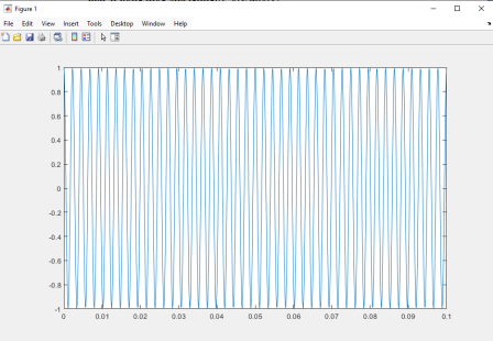
Fig. 3. Cosine function
Indeed, we observe the cosine wave oscillating between -1 and 1. At this stage, we listen to our signal by using the command sound (x, Fs), where we pass our vector x and the sampling frequency Fs as arguments.
Next, we need to create additional sinusoids by defining a vector of center frequencies as Fc= [440,550,660]. This gives us a column vector. Why is it important? We do not change the syntax for generating the sinusoid, we still write x = cos(2 * pi * fc * t). However, in this case, we do not simply multiply the scalar values by the vector. Instead, we multiply the scalar values 2π by both the column vector Fc and the row vector t. The result of the multiplication is the 3×801 matrix, where each row represents a separate sinusoid. By visualizing the matrix in figure 4, we can see three distinct sinusoidal waves.
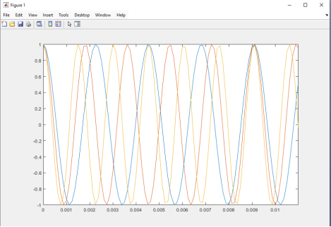
Fig. 4. Three distinct sinusoidal waves
To listen to the chord we need to summarize the three sinusoids together. We can use the built-in sum function, which adds the values across the rows of the matrix. After summing we obtain the row vector. The matrix before and after the addition is shown in figures 5 and 6.
Before:

Fig. 5. Matrix before addition
After:

Fig. 6. Matrix after addition
Now, we need to normalize the resulting vector so that its amplitude range is between -1 and 1. We can verify this by inspecting the variable in the Workspace, ensuring that the maximum value returns to 1.Figure 7 shows signal normalization

Fig. 7. Signal normalization
Next, we visualize it using the plot command. This shows the sum of the three sinusoids in the time domain, which represents how the chord A appears. Figure 8 shows sum of the three sinusoids
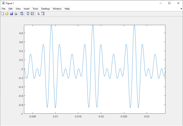
Fig. 8.Sum of the three sinusoids
Using our knowledge of the chord construction, we can play various musical melodies. Below, there is a sample MATLAB code that creates a sequence of chords, inspired by a musical excerpt from Playboi Carti — Location.
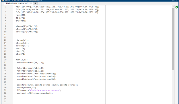
Fig. 9. MATLAB code for musical excerpt
In conclusion, we have demonstrated a systematic approach to synthesizing musical chords using sinusoidal signals. By generating sinusoids based on the central frequencies of notes, summing them to from chords, and normalizing the resulting signal, we archived a clear and reproducible method for creating harmonic structures. Visualization of the chords in the time domain and playback of a chord sequence illustrate the effectiveness of the approach in replicating musical excerpts. This method provides a foundation for further exploration in digital music synthesis of signal processing in musical contexts.
References:
- Upadhyay R. K. Digital Signal Processing: From Theory to Practical Applications // Journal of Propulsion Technology. — 2023. — Vol. 44, № 4.
- Lai E. Practical digital signal processing //. Elsevier. 2003.
- Rao K. D., Swamy M. N. Digital signal processing. Theory and practices // Springer. 2018
- Karl, J. H. An introduction to digital signal processing // Elsevier. 2012
- Proakis, J. G. Digital signal processing: principles, algorithms an applications // 4/E. Pearson Education India. 2007

